Correlation & Causation: Why running in football appears to be useless

The data boom in football lets us answer questions more quickly than ever, scratching deeper and deeper under the surface, uncovering the sport’s messy truths. Some questions are idle curiosities, but many are functional with a deeper question in mind: how do we win more games?

One such question is the effect of running. This is a classic how do we win more games? question. It’s easily measured, and easily coached. Intuitively, it feels right. Try hard, run lots, win games.

However, research over many years has pushed back against that. There is often little correlation found between running more and winning games [1–3]. Many have taken this to mean that running does not have a relationship with winning [1, 4].

This is not true.

In the same way that correlation does not equal causation, a lack of correlation does not equal a lack of causation.

This article makes the case that running is quite obviously important but, more broadly, illustrates issues with asking nuanced questions of coarse data.

---

Suppose that you find a plant in the forest and extract an unknown drug from it. It is unclear what this drug does. In lieu of testing facilities (or research ethics!) you find a thousand people willing to let you test this drug on them.

Five hundred of these brave volunteers carry a variant of gene X which we’ll call Variant A, and the other five hundred carry a different variant which we will call Variant B.

Within a week, each person with Variant A who was given the drug grows six inches taller. In the same timeframe, each person with Variant B who was given the drug shrinks by the same amount.

A control group did not change in height whatsoever.

You check the correlation between the drug and height.

There is no correlation.

Are you safe to assume that there is no relationship between the drug and height?

The answer is, of course, no. There is clearly a relationship.

And, since I engineered the example to make a point, we know the underlying mechanism at play here: this is a causal relationship. The mystical drug causes a change in height that manifests differently based on an interaction with gene X.

So, causation is possible without correlation.

---

Back to football, how much can we really know from a (lack of) correlation between distance covered and results?

The interaction with gene X is a stand-in for tactical context.

There are some research articles that study this explicitly. They separate a match into phases and analyse total distance by phase instead of aggregated over the whole match.

They largely find that, split this way, distance is related to results in different ways [5–7]. That implies that running more is right in some cases, wrong in others, and maybe neutral in the rest.

This is somewhat intuitive.

Football is complex. It would be ridiculous to suggest that simply running more would make everyone in every situation more likely to win.

It might be a cliché, but the only variable we actually care about is goals. All metrics—expected goals, expected threat, whatever else we can expect—are designed to predict goals.

Blindly optimising them without considering the nature of their relationship with actual goals can backfire. For instance, you could consistently go long to your tall striker and have them keep heading it down into awkward positions for their teammates. You’d end up with a high expected threat at the end of a match (as it values geographical progression), but it’s unlikely to translate into many goals if you can’t retain the ball to turn it into a chance.

Similarly, blindly optimising running distance is unlikely to be a magic ‘goals’ button. Sprinting towards the touchline while the other team strolls into your box through the space you just vacated probably isn’t going to help your chances of winning.

However, if your defenders refuse to run while the opposition pump the ball over the top then you’re probably going to end up more likely to lose. In that situation, you probably do want them to cover distance, and quickly!

This is Variant A and Variant B. In one case, the intervention helps and in one case it harms.

Segmenting a match into tactically similar phases can help to capture this effect. Teams perform different physical actions in different tactical phases [8, 9]. In transitions, players are more commonly far from the ideal position and need to run. In settled possessions, teams often take up their desired shapes quite quickly and have a risk of running out of position.

This also leads to confounding. Team quality affects both how often a team wins and how much of the ball it has, and so how much it needs to run. Good teams have the ball more: across five Premier League seasons, possession and points per game are strongly correlated [6]. That means the distribution of these tactical phases by teams is not equal. Good teams are in settled possession more. They therefore have less need to run throughout a match. Over a season, it then looks like good teams aren’t running more. In an absolute sense, maybe they aren’t. But they likely are when required.

The distribution of tactical phases also shifts with game context. The game is not the same when you are winning and losing. If you run more when you have to chase the game [10], we have another issue: reverse causality. Better teams are running less because they are winning more. By 3-0, perhaps you’ve just done all the running you need to.

We’re also looking at a restricted sample. Elite athletes are good runners, and cover lots of distance when playing sports. The differences between teams in the same league are small: in 2025/26, Premier League teams averaged between about 110 and 119 km a match. It is akin to a study on height and basketball performance using only NBA players. You’re only discerning between those at the margin and have no baseline. The difference between 6’6” and 6’7” might not be a lot, but height is obviously important, and the selection process filters by this. Perhaps the same is true of running in football. On top of that, there are only 20 teams in a league, which is very few from a statistical point of view. Only quite extreme effects will be obvious after a single season.

But ultimately, it’s very hard to reach conclusions with such coarse measurements. Aggregating over a match loses information on when the running occurs. We can partially recover this with tactical context. Distance covered also conflates types of movement: walking, jogging, running. Lionel Messi choosing to walk often and sprint rarely [11] is a nice case study into this: running is obviously important, and one of the best players ever has an extremely keen sense of exactly when that is. In the aggregate, it looks like he just doesn’t really move.

---

This is pretty abstract so far, and I might just be making things up. Let’s look at some real data.

FotMob kindly share Opta’s physical data for the Premier League, so we looked at the 2025/26 season’s running data. Some games were missing and their information was only available in the aggregated season totals, but details on this and our robustness checks are at the end of this post in an appendix. TL;DR: it doesn’t really change anything. Any analyses affected by this have a footnote.

So first, let’s just plot out distance covered and points. As you can see below, the correlation is very weak: r = 0.22*. Some teams ran a lot and were good (Manchester City and Arsenal). Some teams ran a lot and were less good (Newcastle, Leeds, Burnley). Some teams didn’t run a lot and were good (Manchester United, Aston Villa). Some teams didn’t run a lot and were less good (Wolves).

*Quick primer if r is new to you: it runs from −1 to 1. At 1, two things rise together perfectly; at −1, one falls as the other rises; at 0, there’s no straight-line relationship at all. With only 20 teams, you’d see a correlation at least this strong about a third of the time by pure chance, even if there were no real relationship, so it’s not statistically significant.

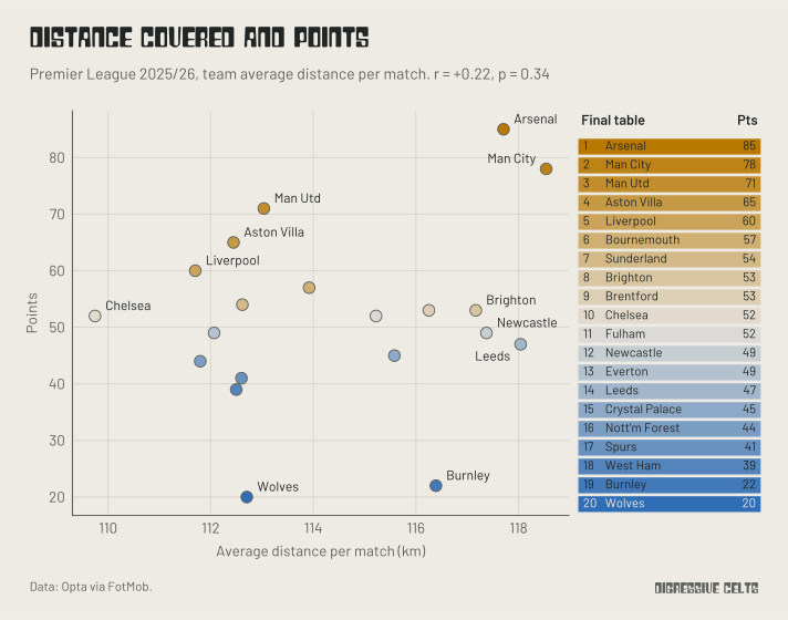
So far, so good. This matches what most previous studies have found on the correlation between distance and points [1–3].

Next, we looked at how distance changed in the second half of games, grouped by the score at half-time: leading, level or trailing. The graph below shows this for both total distance and running distance. In both cases, the change in second-half distance is lowest when leading and highest when trailing. Teams ran more when they were chasing the game.

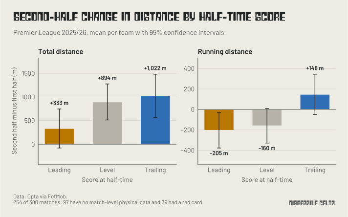
For full transparency, one caveat: second halves tend to have more added time, so every group would cover more distance after the break if all else was equal. That lifts all of the bars, so you can’t read too much into changes versus zero, and bars should be compared to each other instead.

We also checked how distance changed with the winning margin within a game. Essentially, do teams that win by more also cover more ground than their opponents when we zoom into single games? The graph below shows that the correlation with total distance is stronger here than across a season (r = 0.36, against 0.22), and that this is dominated by low-speed movement. Running and sprinting have almost no correlation (r = 0.03 and 0.09).

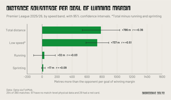
Teams that won tended to cover more ground at low speeds, but they didn’t run or sprint any more. That supports the idea of spending more time in settled possession, where they can pass around and trigger quick (albeit contained) movements from the opposition block, or building up with the defending team pressing harder.

So, we can see that there is an effect. It’s maybe just a little lost in how we’re measuring it.

---

Economists have a neat illustration of this, known as Milton Friedman’s thermostat [12]. Picture a house with a good thermostat. On cold days the boiler uses lots of energy. On warm days it barely turns on. The temperature inside never changes.

Look only at the data and you’d find no correlation between the energy used and the temperature indoors. You might conclude that the boiler does nothing. You would be wrong: the missing correlation is proof, in this case, that it is working as it should.

Footballers are the boiler. Good teams don’t run a fixed amount; they run as much as is required. Sprint back in transitions, hold your shape when breaking down a low block, ease off when you’re cruising. The better a team is at choosing their moments correctly, the less their total distance will line up with their results.

It’s the drug from the start, too. Running helps in some situations and hurts in others, and over a match and a season the two hide an actual effect. The lack of correlation between the drug and height wouldn’t result in anyone claiming the drug was useless. It instead would be a case of determining when it was an appropriate treatment.

Effects can cancel out. They can be hidden by just doing what they should be doing. Football has this, plus a bunch of other contextual bits that change what the ‘right’ thing to do is. Put together, it would be surprising if running and results lined up neatly.

Correlations are great for finding effects in the aggregate, but questions in football often require more specific answers than that. Coarse questions with coarse data give coarse answers: a lack of correlation is not a lack of causation. In this case, it is simply a lack of context.

References

Running and winning

[1] Di Salvo V, Gregson W, Atkinson G, Tordoff P, Drust B (2009). Analysis of high intensity activity in Premier League soccer. International Journal of Sports Medicine, 30(3), 205–212. https://doi.org/10.1055/s-0028-1105950

[2] Allen T, Taberner M, Zhilkin M, Alexander J, Harper D, Rhodes D (2025). Is it as simple as run more, win more? Influence of running load on match outcome and final league position across nine consecutive English Premier League football seasons. International Journal of Sports Science & Coaching, 21(3), 1504–1512. https://doi.org/10.1177/17479541251371004

[3] Poli R, Ravenel L, Besson R (2021). Analysis of the distances covered in professional football competitions. CIES Football Observatory Monthly Report, 68. https://football-observatory.com/IMG/sites/mr/mr68/en/

[4] Premier League (2022, 17 November). Which Premier League team have run the furthest? premierleague.com. https://www.premierleague.com/news/2910649

Phases of play

[5] Hoppe MW, Slomka M, Baumgart C, Weber H, Freiwald J (2015). Match running performance and success across a season in German Bundesliga soccer teams. International Journal of Sports Medicine, 36(7), 563–566. https://doi.org/10.1055/s-0034-1398578

[6] Allen T, Taberner M, Zhilkin M, Harper D, Alexander J (2026). Possession in motion: a five-season analysis of running in-possession and out-of-possession with match outcomes in the English Premier League. Biology of Sport, 43, 899–909. https://doi.org/10.5114/biolsport.2026.159531

[7] Modric T, Versic S, Drid P, Stojanovic M, Radzimiński Ł, Bossard C, Aftański T, Sekulic D (2021). Analysis of running performance in the offensive and defensive phases of the game: is it associated with the team achievement in the UEFA Champions League? Applied Sciences, 11(18), 8765. https://doi.org/10.3390/app11188765

[8] Caldbeck P, Dos’Santos T (2022). How do soccer players sprint from a tactical context? Observations of an English Premier League soccer team. Journal of Sports Sciences, 40(23), 2669–2680. https://doi.org/10.1080/02640414.2023.2183605

[9] Jerome BWC, Stoeckl M, Mackriell B, Dawson CW, Fong DTP, Folland JP (2024). Contextualised physical metrics: the physical demands vary with phase of play during elite soccer match play. European Journal of Sport Science, 24(11), 1627–1638. https://doi.org/10.1002/ejsc.12209

Game state

[10] Lago C, Casais L, Dominguez E, Sampaio J (2010). The effects of situational variables on distance covered at various speeds in elite soccer. European Journal of Sport Science, 10(2), 103–109. https://doi.org/10.1080/17461390903273994

Coarse measurement

[11] O’Neill C (2026, 11 July). Lionel Messi has spent 64% of this World Cup walking — but he is always ready to pounce. The Athletic. https://www.nytimes.com/athletic/7434324/2026/07/11/lionel-messi-walking-world-cup-argentina/

Conclusion

[12] Romanchuk B (2024, 22 January). Why the “Friedman thermostat” analogy should be uncomfortable for the mainstream. Bond Economics. https://bondeconomics.substack.com/p/why-the-friedman-thermostat-analogy

Nick Rowe popularised the analogy in a 2010 blog post, but that was on Typepad, which has since shut down, so this explainer is the best live link.

Appendix: missing data robustness

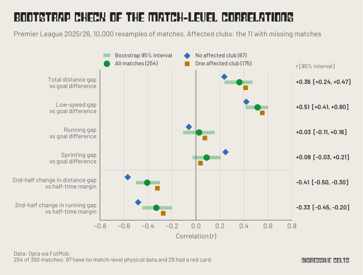
Since some games were missing, we did some checks to make sure that all the effects weren’t carried by a few games or teams. This was to reassure ourselves that recovering the missing games wasn’t likely to swing our results entirely the opposite direction. We found that our results were pretty robust and it’s unlikely the missing games would change anything.

We did 10,000 bootstrap resamples of the 254 (out of a possible 380) matches we used (97 missing, 29 excluded for having a red card). For those not familiar, bootstrapping is where we essentially randomly re-draw from our data samples repeatedly (allowing the same games to be picked multiple times) to estimate uncertainty. In a single bootstrap rep, our full sample of games might include the same game several times or not at all. If single games swing the results wildly, our resulting confidence interval from this process will be very wide. If our effects are robust, the confidence interval will be narrower. Bootstrapping only tells us how much random noise there is in the games we have, though. It can’t tell us whether the missing games are different, which is what the next checks are for.

We also checked what happens if we drop a single team’s data and check correlations without them in case any single team is carrying the effects observed. Then we checked what happens if we don’t use clubs with missing data at all.

The graph below shows our results. In short, none of the clear results changed sign (positive results becoming negative or vice versa); only the running and sprinting correlations, which sit close to zero anyway, flip back and forth. Dropping any single club moved the correlations by 0.10 at most. Using only the 67 matches with no affected club moved them by up to 0.16, but every clear result kept its sign. We also compared some basic information across our sample and the missing games and saw that it was similar: our sample had 44% home wins and 2.76 goals per game, against 40% and 2.71 in the missing games. None of this guarantees that the missing data behaves the same as this, but all of these games exhibiting similar patterns is a good indicator that the effect was robust and little would change with those games added.